Wave Resource Estimation Using DHI MIKE - Retrieving Coastline Data

Contents

• Introduction
• Sourcing Coastlines from GSHHS
• Manipulation using MATLAB
• Exporting to DHI MIKE xyz format

Introduction

This page is a guide for sourcing data that provides cartographic information about the location of coastlines. The page will detail the data sources, and any conversion techniques required to use the data with DHI MIKE.

Sourcing Coastlines from GSHHS

The most cited source for coastline data is provided by The National Geophysical Data Center (NGDC) which is a part of the National Oceanic & Atmospheric Administration (NOAA). The particular data set is called Global Self-consistent, Hierarchical, High-resolution Shoreline Database (GSHHS).

The web address for this data set is here:

http://www.ngdc.noaa.gov/mgg/shorelines/gshhs.html

The complete data set can be downloaded from the above page. The page also contains a link to an extractor which is called GEODAS Software for Windows. Note this software will work only in windows and it requires the WDBII Rivers and Political Boundaries data set to be downloaded in addition to the GSHHS shorelines. The extractor and the WDBII data can both be retrieved from the GEODAS Software page.

Once the program has been installed, start the program called Coastline Extractor in the GEODAS menu.

On first starting of the Coastline Extractor you may have to provide the location of the coastline and boundary data. To do this go the the Coastlines+ menu and select GSHHS Shorelines. You should then be prompted to provide the location of the downloaded and unzipped data sets (I placed these into the GEODAS program directory).

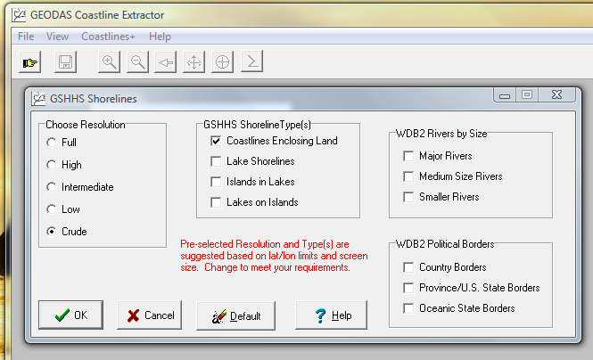
With the data sets selected a coastline can be plotted by selecting the File menu and choosing Plot or by clicking the finger button. You will then be able to select the region of coastline you wish to plot (in longitude and latitude) before being brought to the main options menu as seen below. There are 5 available resolutions which are:

• Full resolution: 0.04 km (~1 arcsecond)
• High resolution: 0.2 km (~6.5 arcseconds)
• Intermediate resolution: 1.0 km (~0.5 arcminutes)
• Low resolution: 5.0 km (~2.5 arcminutes)
• Crude resolution: 25 km (~13.5 arcminutes)

(Information from http://comlmaps.org/how-to/layers-and-resources/physical-environment/gshhs_shoreline)

After choosing a resolution, the type of data required must be selected. For the purposes of wave energy modelling only the Coastlines Enclosing Land option need be checked.

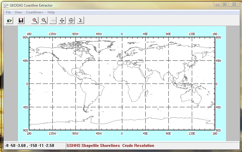
Selecting the entire world at crude resolution should then generate a map like this:

To save the coastline data File > Save As… brings up a number of choices of file format. The MATLAB Coastline Format is useful for preparing data to be imported into DHI MIKE (as discussed below), but other formats may be more applicable to other applications. Choose a format, click OK, and provide a file name and you’re done. If you want to do differing resolutions then just repeat the above for each required grid size. The coastline extractor can’t merge resolutions so this will have to be done using another method.

An older and now depreciated data set can also be extracted via an online form found at:

http://www.ngdc.noaa.gov/mgg/coast/

This might be useful for some alternative resolutions to those provided by GSHHS, although these are all listed using map scales so I’m not sure about comparing the resolution of these sets.

Manipulation using MATLAB

MATLAB coastline format uses NaN terminators to separate distinct coastline segments (see the MATLAB mapping toolbox documentation for more information). Although the GSHHS coastline extractors do their best to produce this format exactly, it can often be the case that certain parts are incorrect. To that end the providers of the GSHHS data have also produced some MATLAB scripts which will fix broken coastlines and remove extraneous NaNs. The scripts can be downloaded from:

http://www.ngdc.noaa.gov/mgg/coast/joincst.html

The downloaded script “joincst.m” is a bundle containing two functions “join_cst.m” and “fixcoast.m”.

Once the coastline data has been imported, “fixcoast.m” will produce new coastline vectors that have a single row of NaNs delimiting each segment and a row of NaNs at the start and the finish.

“join_cst.m” will concatenate segments of coastline that are within a given distance of each other. Thus the command:

[new_coast, slen] = join_cst (coast, 5.)

will joint all segments in the original coastline that have start or end points which are closer than 5 degrees of length in the geographic coordinate system (longitude and latitude). Obviously this would join most islands to coastlines so it’s recommended that the choice of length be less than the resolution of the data set. For the above command, “new_coast” is the joined coastline and “slen” is an array showing the number of points in each segment for the new joined coastline.

Exporting to DHI MIKE xyz format

The following MATLAB script will convert a MATLAB coastline data set into a MIKE xzy file that can be imported for coastline.

function write_xyz(land_data, filename, filter)

% Takes NOAA generated land data and outputs it into an xyz format
% compatible with MIKE.

% Get all the NaNs in the array
data_nan = isnan(land_data(:,1));

% Get the indices of all the nans
nan_ind = find(data_nan==1);

% Open the file for writing
fID = fopen(filename, 'w');

% loop through the indicies.
for k = 2 : length(nan_ind)

    % Check the number of points between the NaNs
    if (nan_ind(k) - nan_ind(k-1)) > 99

        % Write to the file
        start_ind = nan_ind(k-1) + 1;
        end_ind = nan_ind(k) - 1;

        % Filter out every tenth entry
        filt_ind = 1:filter:(end_ind - start_ind + 1);
        copy_point = land_data(start_ind:(end_ind), :);
        ones_length = length(filt_ind);

        fprintf(fID,...
                '%8.5f %8.5f %i %i\n',...
                [copy_point(filt_ind, :),...
                  ones(ones_length,1), 10*ones(ones_length,1)].' );

        % Write the end node
        fprintf(fID, '%8.5f %8.5f %i %i\n', [land_data(end_ind, :), 0, 10]);

    end

end

% Close the file
fclose(fID);

land_data is the MATLAB format coastline data, filename is the name of the file (note the .xyz extension must be explicitly given in the filename) and filter is a method for skipping points if you want to reduce the size of the dataset, i.e. filter of 2 will print every second point.

Again, this script could be a bit more clever than it is (such as including distance filtering rather than the blunt approach above), and centrally managed, but I’ve not gotten around to that yet.

The actual format of the xyz file is quite simple. There are four columns: X, Y, connectivity and Z. The X and Y is positional data of the land and the Z value can be simply chosen as 10 for all points given the points represents land. The connectivity column is used to delineate segments of land. This is done by having a value of 0 for the last point of each segment, whilst the other points all have 1 for this value. An example of part of a file is below:

-47.87250 60.97078 1 10
-47.84023 60.97048 1 10
-47.82498 60.97048 1 10
-47.81853 60.97694 1 10
-47.79828 60.98222 1 10
-47.78420 60.98662 1 10
-47.80181 60.98779 1 10
-47.84170 60.98544 1 10
-47.84493 60.97870 1 10
-47.85520 60.97635 1 10
-47.87250 60.97078 0 10
-3.14916 58.82665 1 10
-3.13830 58.81697 1 10
-3.10428 58.81902 1 10
-3.07905 58.81580 1 10
-3.07758 58.83340 1 10
-3.10340 58.83046 1 10
-3.09753 58.83838 1 10
-3.06849 58.84953 1 10
-3.11836 58.84542 1 10
-3.13830 58.83633 1 10
-3.14916 58.82665 0 10

So here we have two segments of land, both containing 11 points.