Better zero crossing estimation for fifthwave

Had some difficulties getting decent zero crossing approximations for fifthwave. The main issue is that the data generated from the Starccm+ plots is quite messy in that it is rather zig-zaggy having some points very close to others, but not coincident or even the direction you might expect.

This has caused a number of problems with the code in the past (particularly when estimating wavelength and celerity which relies on good estimation of the zero crossings). The original code had a basic linear interpolation routine checking for a switch of sign and them some error checking after that to make sure it wasn’t an inflection. Unfortunately the messiness of the data made this process extremely unreliable.

Moving onto examining all the waves in the numerical wave tank (NWT) rather than just a region of it required much better estimation of the zero crossings in order to strongly identify which wave was which after a time step and thus, monitor its progress. I needed to smooth the data before it could be really useful and then best solution to this would seem to be splines.

Spline fitting is a pretty heavy bit of mathematics, but I am lucky that the authors of Scipy (the scientific Python library) created an interface to FITPACK (a FORTRAN curve fitting library) called scipy.interpolate. Thus generating splines was not too difficult, it’s just deciding what to do with them. This takes me on a slight tangent where I must express the discomfort caused by using something you don’t understand and the risks associated with that. I have a mathematics degree, but not enough time to learn splines again so I just merrily let the smoothing routine do it’s business and harvested the neat roots() method which gives the roots of the spline (or the zero crossings. Only until the results continued to be a bit rubbish did I actually investigate what was going on and this is what I found.

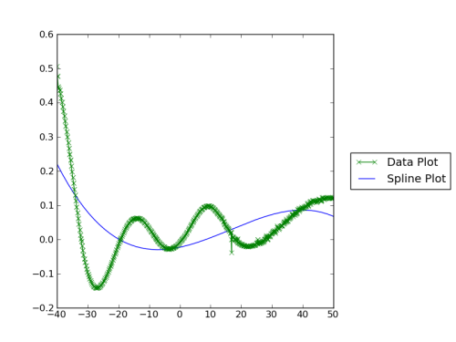
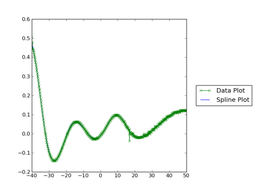
Basically the default spline is absolutely nowhere near the wave form. The smoothing parameter ‘s’ was set way to high (in fact, if it’s not specified its the length of the data i.e O(1000)). Ideally the smoothing in this first case should be O(0.01) which generates a results like this:

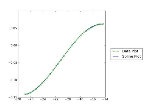
Close up though this still isn’t perfect and it may be that it won’t calculate this level of smoothing which means that I want to reduce the amount of data that the spline is fitted to, idealy to go from peak to trough to peak. To get a good estimate of the locations of the peaks and troughs, I create another graph of the 1st derivative of the above spline and fit another spline (with even lower s this time) and find it’s roots. This gives me the turning points of the original data. I do need to be careful here, however, as I want to get peak trough, so if there is another peak in there, I skip it till I find a trough. Finally I trim the data to a region between a peak and trough and fit a new spline (default smoothing is fine now), and voila, a good approximation to the zero crossing can be found. Here’s one I made earlier.

Finally, I’ll just put a quick summery of the code for getting these plots, etc, so that I can do it again if it all goes a bit airy.

# Import the fifthwave module
import fifthwave as fw
from numpy import linspace

# Set up the wave form data from a csv file
test_data = fw.TwoD_Wave_Form()
test_data.import_csv('mycsv.csv')

# Fit the first spline to that data and plot it
test_data.fit_spline(smoothing=0.01)
test_data.spline_plot('first_spline.png')

# Now build another wave form based on the gradient of the first spline
new_x = linspace(test_data.x[0], test_data.x[-1], len(test_data.x))
new_eta = test_data._spline(newx, 1)

work_data = fw.TwoD_Wave_Form(eta_list=new_eta, x_list=new_x)

# Get the spline approximation and the roots.
work_data.fit_spline(smoothing=0.001)
work_data.spline_plot('gradient_spline.png')

inflections = work_data._spline.roots()

# You can now filter the inflections to make sure they run peak to trough
# Finally for each inflection move the work data and find the root, i.e there
# may be a crossing between the start of the data and the first inflection
fromindex = 0
toindex = test.closest_x(inflections[0]) + 1

work_data.x = test_data.x[fromindex:toindex]
work_data.eta = test_data.eta[fromindex:toindex]

work_data.fit_spline()
work_data.spline_plot('final_spline.png')

print 'Zero crossing is at ', work_data._spline.roots()[0]

# Note that the current smoothing factor is not easy to recover from the
# spline, but in fact it is given by
test_data_spline_smoothing_factor = test_data._spline._data[6]